What Is AMS Verification? RNM, Co-Simulation and UVM-MS Explained

Analogue/mixed-signal (AMS) verification checks that a design containing analogue behaviour and digital logic operates correctly, particularly where voltages, timing, control decisions and operating states interact. Unlike digital-only verification, it must account for physical quantities and tolerances as well as discrete logic values. Engineers use behavioural models to represent selected analogue effects, real-number modelling (RNM) to exercise those effects in digital-centric simulations, and AMS co-simulation when analogue and digital simulation domains need to interact. Accellera’s UVM-MS methodology provides a structured way to drive and monitor mixed-signal interfaces from a UVM environment. These approaches are complementary: the appropriate combination depends on the verification question, required fidelity and evidence available to validate the models. [1–3]

What Is AMS Verification?

An AMS design combines circuitry whose behaviour depends on analogue quantities with digital functions that configure, sequence or interpret that behaviour. Examples include an analogue-to-digital converter (ADC) controlled by registers, a DAC driven by digital samples, a phase-locked loop (PLL) with a programmable divider, a power-management block with digital mode control, and a sensor front-end that reports measurements to a processor.

Verification therefore has to check more than whether a register write is legal or a digital state machine reaches its expected state. It may need to establish whether an analogue signal has settled before sampling, whether a digital result represents the intended input range, whether a change in reference voltage is handled correctly, or whether a power-mode transition invalidates an in-progress conversion. A correct digital sequence can still give the wrong result if its assumptions about analogue response are false.

The important boundary is what the test proves. A digital-only model may establish protocol ordering and register behaviour but omit actual settling. An abstract analogue model can check selected voltage and timing relationships, but does not automatically establish transistor-level noise, linearity or process-voltage-temperature (PVT) performance. AMS verification combines appropriately scoped checks rather than expecting one model to prove every property.

How Does AMS Verification Work?

A practical verification flow starts with an explicit requirement and finishes with evidence that can be reviewed against that requirement:

Requirements and operating modes → model selection → stimulus → simulation → observation → independent checking → coverage and review.

First, engineers identify the behaviour to check: for example, after the controller requests a conversion, the ADC returns a valid code only after the specified completion condition. The verification plan records relevant modes, analogue operating limits, timing constraints and expected outcomes. It should also state which model is permitted to support which check.

Next, the environment represents the design at a useful level of abstraction. A digital controller might be RTL, while its ADC is a calibrated behavioural or real-number model. Another configuration may retain the controller RTL and connect it to a Verilog-A/Verilog-AMS or circuit-level ADC model. The two configurations answer different questions; using both can be appropriate.

The testbench drives digital configuration and analogue stimulus, observes the analogue input at the relevant sampling instant, captures status and output transactions, and compares them with an independent expected-result model. Independence matters: simply calculating the expected value using the DUT’s own output, or copying the DUT’s incorrect conversion algorithm into the reference model, can conceal a design error.

Checks can be exact where the specification and abstraction are deterministic, or tolerance-based where analogue error bounds are defined. Coverage then asks which input regions, modes, reset conditions, timing boundaries and combinations were actually exercised. Passing a regression establishes evidence for those tests and models; it does not, by itself, establish the physical accuracy of every underlying analogue assumption.

For deeper discussion of what happens when interface assumptions and model responsibilities are left unresolved, see AMS Verification Challenges: Why Mixed-Signal Programmes Still Fail Late. This guide concentrates instead on the verification mechanics.

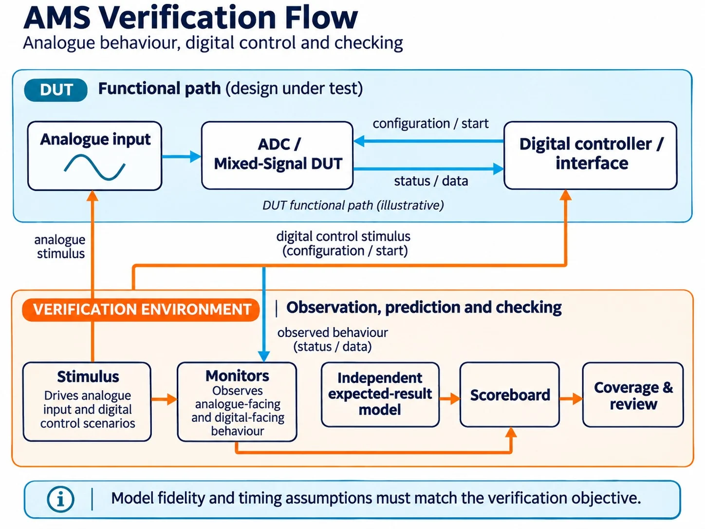
Figure 1: AMS verification flow: analogue behaviour, digital control and checking. The DUT’s analogue conversion and control paths are separated from the verification environment’s stimulus, observation, independent expected-result modelling, scoreboarding and coverage review.

RNM vs AMS Co-Simulation – When Should Engineers Use Each?

Real-number modelling (RNM) is a modelling technique: selected analogue quantities are represented by real-valued variables, nets or related constructs, often evaluated with event-driven digital simulation. Such models can represent transfer functions, finite settling approximations, saturation, reference changes or selected timing effects if they are intentionally implemented. SystemVerilog real values and user-defined nettypes, as well as Verilog-AMS wreal constructs, are examples of implementation choices; their semantics and tool support differ. [3, 4]

AMS co-simulation is a simulation/integration approach: analogue and digital modelling domains are coordinated so that their interactions can be exercised in one environment. Depending on the configuration, the analogue side may comprise behavioural equations or transistor-level circuits. RNM may also participate in a hybrid flow; RNM and co-simulation are not mutually exclusive alternatives. [4, 5]

The right question is therefore not “Which is more accurate?” but “What behaviour must be observed, at what fidelity, and against which reference?” For register-programmable conversion ordering, a well-validated RNM model may be adequate. For a reference-buffer settling fault that changes the conversion result, a transient analogue model may be essential. SPICE-level analysis remains important for device and circuit properties not established by higher-level models.

Cadence describes the role of RNM in digital-centric mixed-signal verification; Siemens documents complementary event-driven and continuous-time mixed-signal simulation options. Neither source establishes a universal speed-up or fidelity guarantee for every flow. [3, 5]

Engineers seeking hands-on practice with these model and simulator choices can explore Alpinum’s AMS Co-Simulation (RNM & UVM) Training.

What Is UVM-MS and How Does It Support AMS Verification?

UVM-MS is Accellera’s mixed-signal methodology extending the class-based approach of UVM (IEEE 1800.2) to interaction with mixed-signal design interfaces. Accellera approved UVM-MS 1.0 for release on 4 February 2025. It is an issued Accellera standard, not a proposed future specification. [1, 2]

Conventional UVM agents use sequencers, drivers and monitors to create and observe transactions. UVM-MS adds a standardised MS Bridge concept for mixed-signal interaction. The bridge is a SystemVerilog module containing a bridge core and an MS Proxy mechanism: the proxy exposes an API to the UVM side, while the core performs the signal manipulation or type conversion needed by the DUT interface. A conventional SystemVerilog interface can also carry supported digital signals. The particular bridge-core abstraction can vary; not every purely digital connection needs a mixed-signal bridge. [1]

For example, a verification sequence can specify a ramp or voltage level. A mixed-signal driver can communicate the relevant parameters through the bridge mechanism; a monitor can measure the response and publish an observation for checking and coverage. The scoreboard then tests the result against a specification-derived expectation. The methodology formalises these interactions without requiring UVM itself to become an analogue simulator.

Three qualifications matter. First, UVM-MS does not create a physically valid analogue model: the engineer still defines and correlates that model. Second, the standard does not guarantee that every simulator and language combination implements each feature; tool-version and interoperability checks remain necessary. Third, UVM-MS is the formal Accellera standard name. The label UVM-AMS, used in some industry or training material, should not be treated as automatically identifying the identical specification or implementation. [1, 2, 6]

Practical Example – Verifying a Mixed-Signal ADC

Consider an illustrative 12-bit, unipolar ADC connected to a digital controller. The controller programs an enable bit and conversion mode, asserts start, waits for done, and captures the 12-bit output code. This is a hypothetical verification exercise, not a claim about a particular Alpinum customer design or a complete production SAR ADC.

1. Define the conversion contract

Assume an ideal straight-binary transfer over a 0 V to 1.0 V input range. For this example the ADC samples the input at the specified conversion-start sampling event; the sampled value remains fixed for that conversion. Its ideal quantisation convention is truncation towards zero for a non-negative scaled input, and its output is saturated to the range 0–4095:

Illustrative ideal transfer: code(Vin) = min(4095, max(0, floor(4096 × Vin / (1.0 V)))).

The ideal LSB width is 1.0 V / 4096, approximately 244.14 µV. At an assumed sampled input of 0.625 V, the expected digital result is 2560 (0xA00). At or above 1.0 V the code saturates at 4095; below 0 V it saturates at zero. These values follow from the specified idealisation, not from a measured circuit. The handling of a real ADC’s over-range behaviour, sampling aperture, offset, gain and noise must come from its actual specification.

2. Drive and observe one conversion

The test starts in a known reset state, enables the ADC, sets a selected conversion mode and applies 0.625 V. It holds the voltage stable across the model’s defined sampling instant, issues start, and records the effective configuration and sampled voltage. If the ADC exposes busy, the monitor checks the corresponding progression; done must arrive within the allowed timing window specified for that mode. The controller must not consume a result prematurely.

At completion, the output monitor captures the code, validity status and completion timing. The reference predictor applies the ideal equation to the recorded sampled voltage and configuration. The scoreboard compares the reported code with 0xA00 and separately checks the control protocol and completion window. Using the voltage at done instead of at sampling would be wrong if the input changed during conversion.

This example intentionally separates analogue correctness (the input-to-code relationship under stated assumptions), digital correctness (configuration, start, busy/done and data acceptance), and testbench correctness (whether the expected value was derived from independent, time-aligned observations).

3. Extend the scenarios without overclaiming

Tests should cover zero and full-scale regions, points immediately either side of code boundaries, representative mid-range inputs, and inputs outside the nominal range where the contract defines the response. Cross these with reset, enable and conversion modes. Exercise start while busy, reset during a conversion, and reference or power transitions only if the implementation specifies their behaviour. An undefined stimulus/response combination should be flagged as a specification gap rather than silently assigned an invented result.

For an ideal RNM model, exact code comparisons may be legitimate. If the model deliberately represents input-referred offset, gain error, settling or reference variation, the checking policy must use explicitly specified error budgets, potentially including code and timing tolerances. Merely allowing a broad numerical margin would reduce the checker’s ability to detect faults.

4. Decide when the RNM result is not enough

A simplified RNM conversion cannot on its own establish capacitor mismatch, comparator noise, reference droop, input sampling dynamics, analogue start-up or PVT-sensitive conversion accuracy. For those questions, correlate the abstract model’s transfer, latency and state assumptions with higher-fidelity analogue simulations or other approved characterisation evidence. Run targeted co-simulations where a circuit-level mechanism and digital sequencing must be exercised together. A successful RNM regression supports only the properties captured by the abstraction and checked by the testbench.

Where Power-Aware AMS Verification Fits

Power-aware verification adds an important class of cross-domain questions: what happens when power is removed, restored or changed while digital control and analogue state are active? Engineers may need to test reset ordering, isolation of unpowered outputs, level-shifter behaviour, reference and bias start-up, analogue settling before the first valid conversion, and control logic that releases an ADC too early.

IEEE 1801-2024, commonly associated with UPF (Unified Power Format), provides a standard mechanism for expressing power intent such as domains and power states. It does not by itself specify the analogue behaviour of a reference, bias circuit or ADC during recovery. Those effects still require suitable analogue models and explicit checking. [7]

Alpinum’s AMS Co-Simulation (Power-Aware / UPF) Training develops this more specialised connection between power intent and mixed-signal verification.

Choosing a Verification Approach for a Mixed-Signal Design

Start by writing down the property to be verified, then choose the least costly model that can actually represent and substantiate it. A useful engineering review asks:

• Observable behaviour: Is the property register ordering, conversion code, analogue settling, supply disturbance, or something else? At which pins, signals or timestamps will it be checked?
• Fidelity and tolerances: Which transfer, timing, non-linearity, noise and PVT effects must the model reproduce? What quantitative error bound is acceptable?
• Control complexity and regression scale: How many modes and sequences need exercising, and can an RNM or behavioural model efficiently cover them?
• Correlation: Which circuit simulations, measurements or specification calculations substantiate the model’s transfer and timing assumptions?
• Tool interoperability: Are the relevant SystemVerilog, Verilog-AMS, real-valued net constructs, bridge mechanisms and simulator versions supported in the selected environment?
• Reviewable evidence: Are the stimulus, monitor observations, scoreboard results, relevant coverage and model limitations traceable to requirements?

Choose RNM for high-volume checks whose meaningful analogue behaviour can be adequately abstracted; use AMS co-simulation when the interaction requires coordinated analogue and digital behaviour; retain detailed analogue or transistor-level verification for properties that need its fidelity. It is normal to use more than one approach at different stages and for different requirements.

Conclusion

AMS verification is effective when the verification question, model fidelity and checking evidence match. RNM makes selected analogue behaviour practical in digital-centric environments; co-simulation coordinates analogue and digital domains where their interaction matters; and UVM-MS offers a standardised way to extend UVM components to suitable mixed-signal interfaces. The ADC example demonstrates the essential discipline: define assumptions, capture the correct analogue sampling event, predict independently, check digital sequencing and investigate limits using more detailed models where needed.

References

1. Accellera Systems Initiative, Universal Verification Methodology for Mixed-Signal Standard (UVM-MS) Version 1.0, January 2025. https://www.accellera.org/images/downloads/standards/uvm-ms/UVM-MS_1.0.pdf
2. Accellera Systems Initiative, Accellera Board Approves UVM-MS 1.0 Standard for Release, 4 February 2025. https://www.accellera.org/news/press-releases/408-accellera-board-approves-universal-verification-methodology-for-mixed-signal-uvm-ms-1-0-standard-for-release
3. Cadence Community, Real Number Modeling Streamlines Mixed-Signal Verification, 24 June 2024. https://community.cadence.com/cadence_blogs_8/b/fv/posts/real-number-modeling-streamlines-mixed-signal-verification
4. Cadence, Solutions for Mixed-Signal SoC Verification Using Real Number Models (established concepts; older white paper). https://www.cadence.com/content/dam/cadence-www/global/en_US/documents/solutions/mixed-signal-verification-wp.pdf
5. Siemens, Questa ADMS analog and mixed-signal simulation (product-specific co-simulation architecture). https://www.siemens.com/en-us/products/ic/questa-one/adms/
6. Accellera, UVM-MS Working Group: Charter and Scope. https://www.accellera.org/activities/working-groups/uvm-ms
7. IEEE Standards Association, IEEE 1801-2024: Standard for Design and Verification of Low-Power Energy-Aware Electronic Systems. https://standards.ieee.org/ieee/1801/7466/

FAQs